M5 Forecasting Accuracy Competition
In spring 2020, during lockdown, I participated in the M5 Forecasting Accuracy competition on Kaggle. Almost a year after the beginning of the competition, I realized that I didn’t talk about it and I didn’t share my code. Most of the solutions shared on Kaggle are in Python, I thought it can interest R users who want to build a forecasting model to see an example in R.
What is the M5 competition ?
The M-competitions are organized by Spyros Makridakis to evaluate and compare different forecasting methods on real world problems. The first competition took place in 1982, with 1001 time series, followed by a competition circa every decade up to the M4 in 2018 with 100 000 times series, and the use of Machine Learning algorithm which performed poorly compared to statistical methods or hybrid using both statistical and ML.
The 5th edition of the M-competitions took place during 4 months from March 3rd to June 30th 2020. The data are provided by Walmart, and consist of 3049 items from 3 categories and 7 departments, across 10 stores in 3 different states, resulting of 30490 hierarchical time series provided by Walmart, with 1941 days of history.
The goal of the M5 competition is to forecast 28 days ahead for all items, and at different aggregation levels (state, store, category, department, state/category, state/department, store/category, store/department etc.) resulting of a total of 42840 times series.
Here is the view of the hierarchy, click on the nodes to expand the sublevel :
One of the particularities of this competition is the evaluation metric. The accuracy is evaluated by the Root Mean Squared Scaled Error (RMSSE), weighted by the cumulative actual dollar sales, based on the 28 last observations. This is justified to give a higher importance to the series that represent higher sales. On the downside, it’s a metric that is difficult to use as an objective function especially when breaking down the data to train different model per store for example.
So the 3 main characteristics of the M5 Forecasting Accuracy competition:
- Hierarchical times series
- Intermittent sales (low level of sales with many days without sales)
- Evaluation metric WRMSSE (Weighted Root Mean Squared Scaled Error)
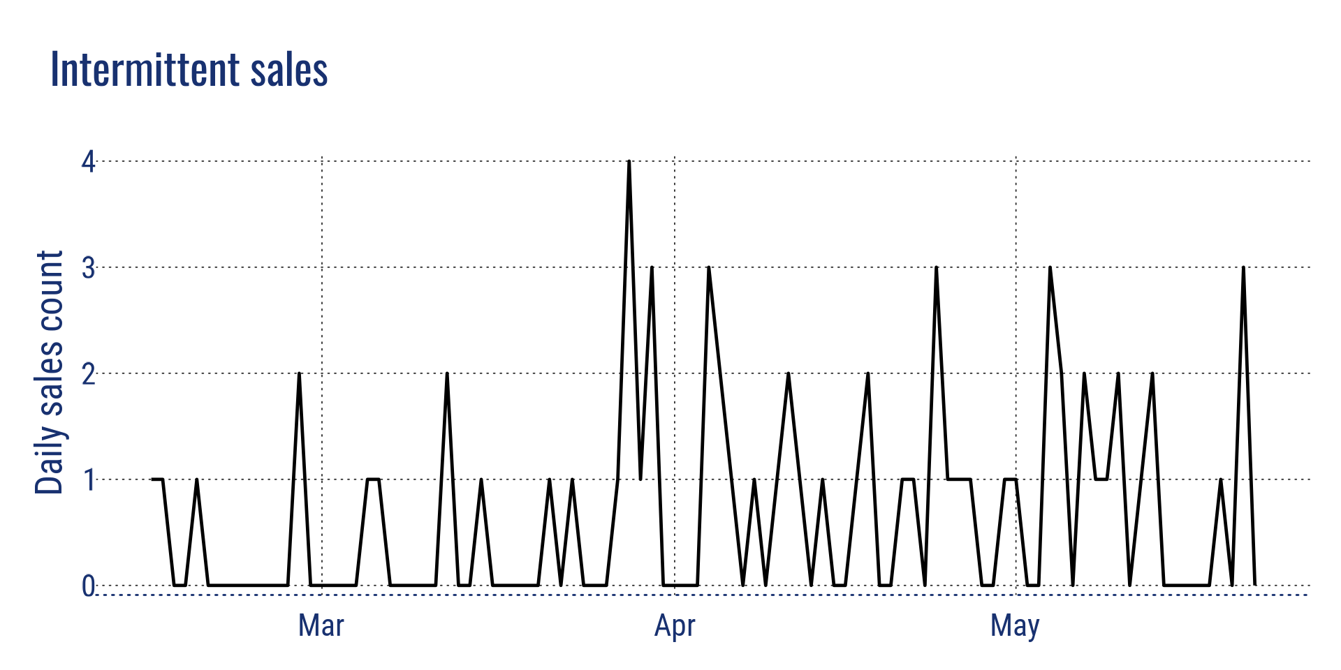
Intermittent sales
The competition had two phases :
- First the validation data were available, with history from 29/01/2011 to 2016/04/24, to forecast for the period of 25/04/2016 to 22/05/2016 (validation period used for the public leaderboard).
- The 1st of June, the real values for the validation period where released, which we could use to analyse and evaluate our model, and to forecast the next 28 days from 23/05/2016 to 19/06/2016, which is the period that is evaluated for the final score in the private leaderboard.
Overview of my work
Quick note
Below, I will explain the principles I used, the difficulties I faced in my environment, which may not apply to yours, and how I solved them, in order to understand better how the code works if you want to experience it. So this article is not a tutorial on how to win a Kaggle competition, or an analysis of the best way to win the M5 competition, but a note on my experience and a guide to understand the code I released.
First steps
I used the competition to experience with different technics and algorithms. After an exploratory data analysis, I started with a naive model, using the data from the previous month, mixed with data from the previous year, to have a baseline for the score, this model gave a WRMSSE of 0.93946.
Arima models where not performing well on intermittent time series, and were very long for 30490 times series, I abandoned them quickly, as well as exponential smoothing which gave few room for improvement. I focused only on gradient boosting decision trees, with XGBoost and LightGBM first, and only on lightGBM as it was performing better.
Technical challenges
The first approach was to build one model, trained on the full data, that would forecast the 28 days for all time series at once. I quickly had a memory issue with this approach. I could only use Kaggle kernel or my laptop, which both have a memory limit of 16 Gb. 30490 time series with 1941 days of history gives a dataframe with 59,181,090 observations. It was only possible to create few new features before exceeding the memory limit, which made it difficult to improve the model.
Another difficulty that I wasn’t expecting, is that the result using Kaggle Kernel were completely different (worse) than running on my own computer. I used the data from a public kernel in Python, using the same exact features and hyperparamaters than the Python kernel, and got a similar score on my machine, but a very bad score when it ran on Kaggle. So I didn’t trust the Kaggle version of LightGBM for R, and decided to use only my laptop.
So, these two difficulties are part of the choices that lead to the final solution:
- Conceptual choices:
- Split the data and build a model by split
- Create an automation, as I execute on my laptop, I need to experience on a single split, and run automatically at night for all the split (approx 8 hours).
- Technical choices:
- Use tidyverse for the features based on the split data, and data.table for the features based on all the data, as data.table update by reference using less memory.
- Save variables to disk for later use, and remove them from memory
- Not using a ML framework in order to control the memory usage, which force to dive deeper into LightGBM to code all the steps.
How it works
The code and the steps to run it can be found on my github repository :
The core of the model
Split by store
The data are split by store_id, which means that there are 10 models for each period (validation & evaluation), so to get a full submission there are a total of 20 models, which generate 20 files that needs to merge into the final file submission.
With this approach, I could deal with the memory issue. However, the model would miss information coming from the rest of the data, for example the volume of sell for this item at the state level, the average sell for that category across all the shops etc.
So I have created a separate script that create the features based on all the data once, that are added to the data for the current split at the end of the feature engineering process for the store.
Weekly forecast
I used a weekly forecast, so I will use some data from the previous week to generate features for the prediction of the current week. The main reason for that, is that the sales are more correlated to the sales of the previous week, than the previous month. There is a big problem with that though. As we have to forecast for 28 days, 4 weeks, the first week will use the true value from the previous week. The second week uses the true values for the features that are with a lag > 7, but has to use the predicted values for the features with a lag < 7, increasing the uncertainty, and leading to less accurate forecast for the following weeks.
To lower the impact, all the features based on the previous week are rolling features using at least a window of 7 days, to smooth the predictions. So the predictions are not used directly as a lag value which would give it too much importance when training the algorithm, and being too inaccurate to predict, but they are used to construct rolling features over a period of 7, 14, 28 days.
The lag values are used directly only with the real values (lag > 28).
Also, for the prediction of each week, I needed to re-calculate the weekly features using the forecast for the week n-1, which is done by the prediction function. So if you use this code and change some weekly features, think about adapting the code in the prediction function as well, otherwise these features will have only NAs.
I thought it was interesting to use this technique because it can apply to business cases when you need more accurate forecast for the firm horizon, and update the forecast periodically.
Here a visual explanation for the 28 days weekly forecast on a single item :

weekly forecast explanation
This weekly forecast is the reason why we see a difference of the RMSE between the data use for validation during the training process (which use the features based on the true values for the past week) and the prediction for the same period using the weekly forecast which recreate the feature using the prediction.
For example in the store CA_4:
- RMSE during validation: 1.33
- RMSE predicting weekly on test: 1.39
- RMSE on new data: 1:43 (calculated after the release of the true values)
So you should rely more on the RMSE based on the weekly prediction which will be closer to what you can expect for the prediction on new data.
Feature engineering
As I explained above, there are two types of features :
- The features created using all the data at different aggregation levels. They are created by a separate script once, and used for each model
- The features created at the store level, that are created for each split.
The features are based on :
- lag values for lag > 28 days, and rolling function with different window size
- rolling mean and rolling standard deviation for the lag values < 28 days with different window size
- features based on calendar such as day of the week, is it a weekend?, holidays, month, special event
- release date of the item
- price features, min, max, mean, sd, normalized, difference in price with previous day, number of shop with that price
- mean encoding
- various statistics
The features created on the whole dataset are mainly mean encoding feature for the different aggregation levels.
You can play with it and add new features, just keep in mind to adapt the prediction function to recalculate them if you modify a feature that uses a lag < 28 as discussed before.
Hyperparameters
I did a hyperparameter tuning with a “poisson” objective, which was doing ok. But after trying another set of parameters suggested by some teams on Kaggle, I used the same hyperparameters that were performing better.
The objective used is a “tweedie” objective, which is more suitable for a distribution with intermittent sales with many zero values. The Poisson distribution is a particular case of a Tweedie distribution with a power = 1.
I used two set of hyperparamaters as I found that the forecast was better with a power = 1.1 on some stores and better with a power = 1.2 on others.
I used a simple RMSE for the metrics, as it simpler to use and interpret, and I couldn’t use the WRMSSE with a model per shop. I found that it was evolving in the same direction than the WRMSSE most of the time. So when I improved the model and got a better RMSE, most of the time the WRMSSE improve too when I submitted the forecast (not in the same proportion though).
Cross validation
Due to the time it takes to train the models on all stores (8 hours), I used a simple train / test split to test new features, and improve the model. A k-fold cross validation would have taken too much time (I needed my computer to work too).
However, every few submissions I did test the consistency of the model by training and predicting on other periods. You can easily adapt the training and test period with two parameters “test_date” and “valid_date”.
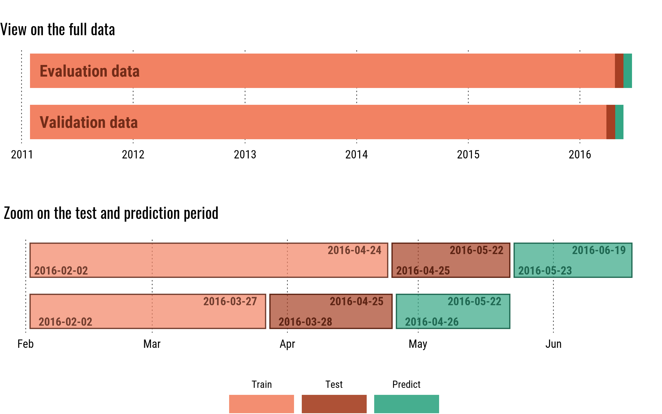
cross validation period
Output
Interactive version
The interactive version that you run in RStudio will give the following ouputs :
- The RMSE for the test data
- The RMSE for the validation data
- The learning curve
- The feature importance
- An interactive plot with the true values and predictions for all departments of the store on the validation dataset
- An interactive plot with the predictions for all departments of the store on the evaluation dataset
Below are some exemple for the store CA_4, you can click on the images to view full size.
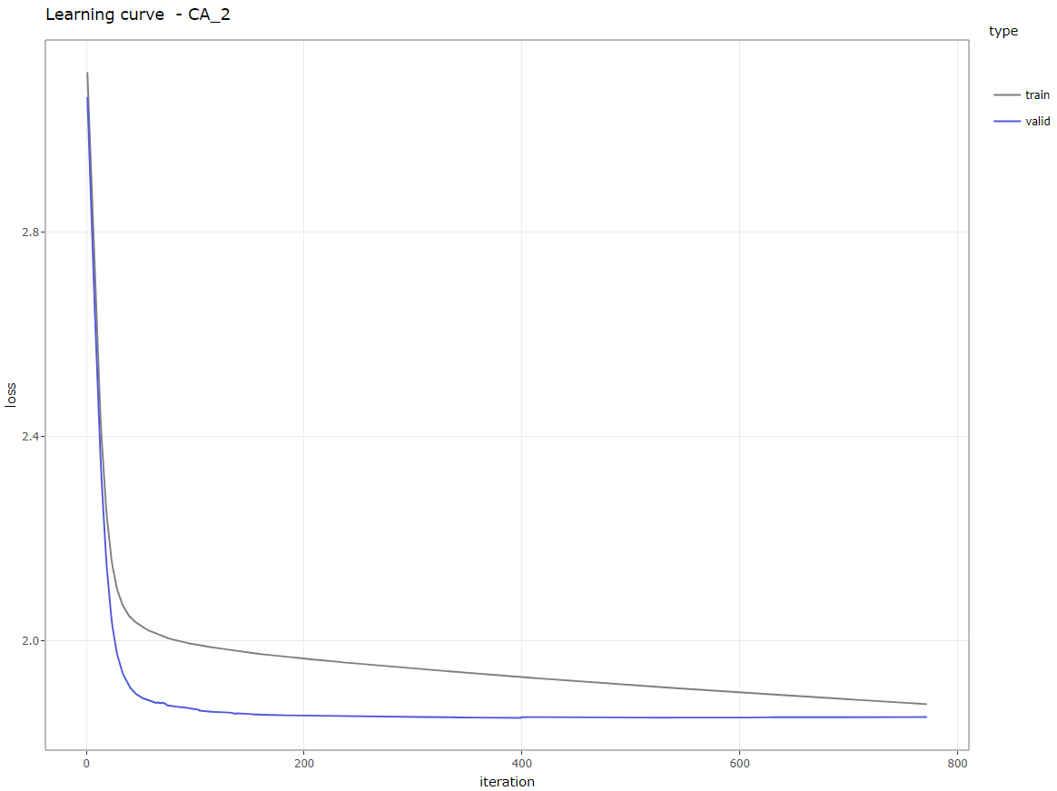
Learning curve
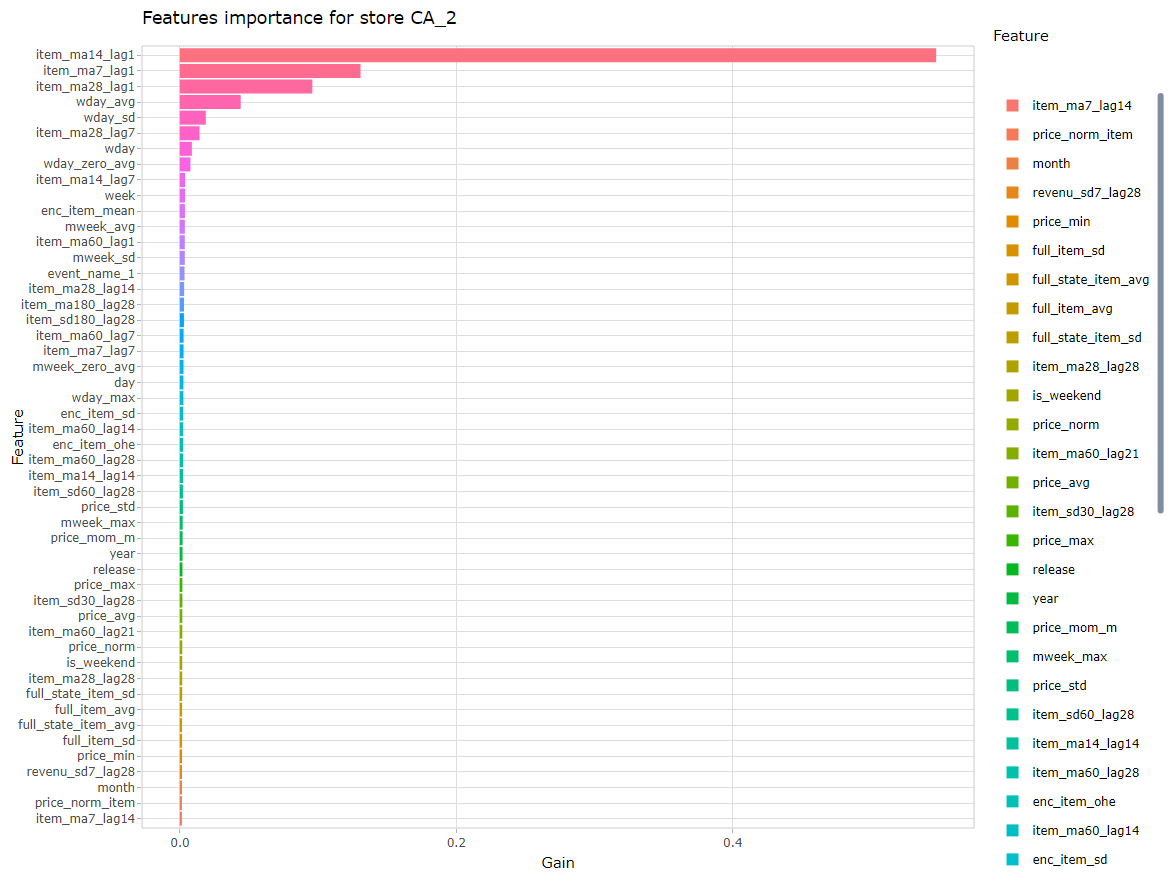
Features importance
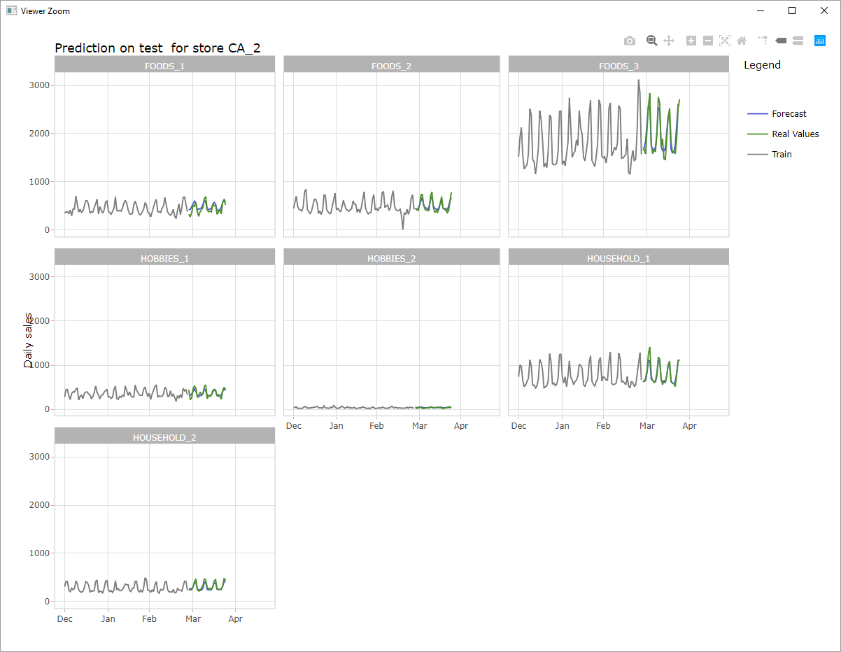
Forecast for all departments
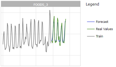
Zoom on one department on validation
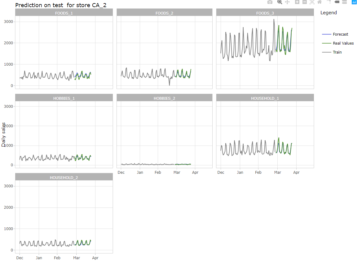
Forecast for all departments
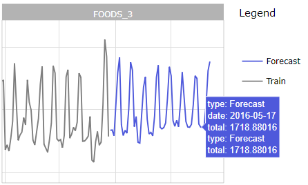
Zoom on one department on evaluation
The script also print in the console many information to know which is the current step in the program.
Automated version
The automated version print the same information in the console to make it easier to check regularly how the program is doing.
It also write a file performance_xx_x.csv with the RMSE for each store and a file features_xx_x.csv with the feature importance (where xx_x is the store_id).
How to run it?
All the steps required to execute the scripts to train the models, predict the forecasting period and merge the forecast are explained in detail on my github repository.
The data are to download on Kaggle or on the competition repository, the links are at the bottom of this article in the “references” section.
Algorithm
Below is a simple description of the algorithm:
Note 1: For this forecast, all the data (except the values to predict of course) are know in advanced. It’s the same states, stores, categories, departments, items, and all the calendar and prices data are available for the next month, which is the period to predict. Therefore, it’s possible to do the feature engineering on all the data, before the split between test and train, and use the same dataframe for validation and evaluation. This is why I can save and load the data for both period, instead of re-executing the feature engineering part.
Note 2: You can retrain the data on the full dataset (up to 2016-05-22) before predicting, or use the model trained on the test dataset (leaving on month gap). The second method worked better for the evaluation period, and is faster as the model is also trained only once. To use the first method, un-comment the corresponding part in the main section of the script.
Results
Competition score
This solution as-is on the github repository gives a Public Score (WMRSSE) of 0.48734 and a Private Score of 0.62408, which would give a position of 190th on 5558 participants, which is in the top 4% and a silver medal for this competition. It’s the state of the model from the last submission I did the last day of the competition.
Usually on Kaggle’s competition, we are allowed 2 submissions, and we can submit a aggressive one and a more conservative one. Unfortunately for this competition, there was only one submission allowed, and I decided to use a previous submission which had a better score on the public leaderboard (0.46744), but it didn’t do as well for the private score : 0.66695, which is the 385th place on 5558, which is in the top 7% and a bronze medal.
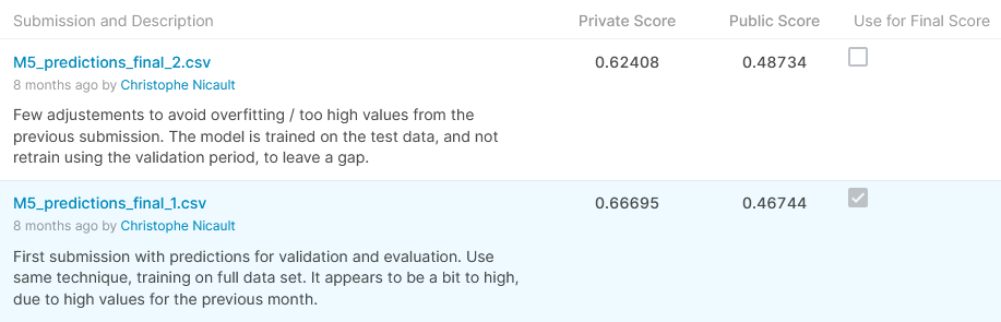
Score on Kaggle
There was a huge shake-up for this competition with different results between the public leaderboard and the private leaderboard. Part of it can be explained by the difference for this period compare to the previous years. For the 5 previous year, the sales in June have always increased compared to the sales in May. The trend was up during the previous month, and most of the model were being optimistic on the volume of sales. For the validation period, many teams used a multiplier coefficient to reflect the trend in the forecast, leading to a better score for the public data, but working only for that period.
Visualisation at different levels
Below are some visualisations to look at the forecasts compared to the real values, at different aggregation level. The real values were disclosed after the competition ending.
Aggregation at state level for California and at store level for store CA_2
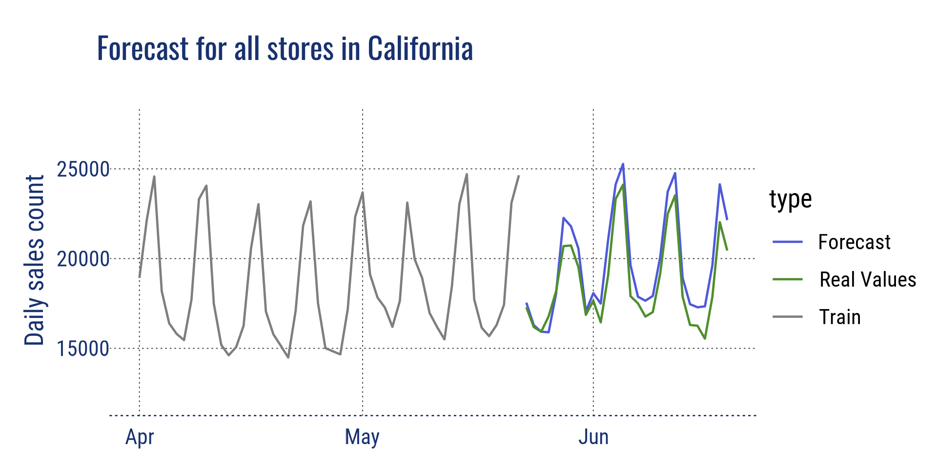
Forecast for all stores in CA
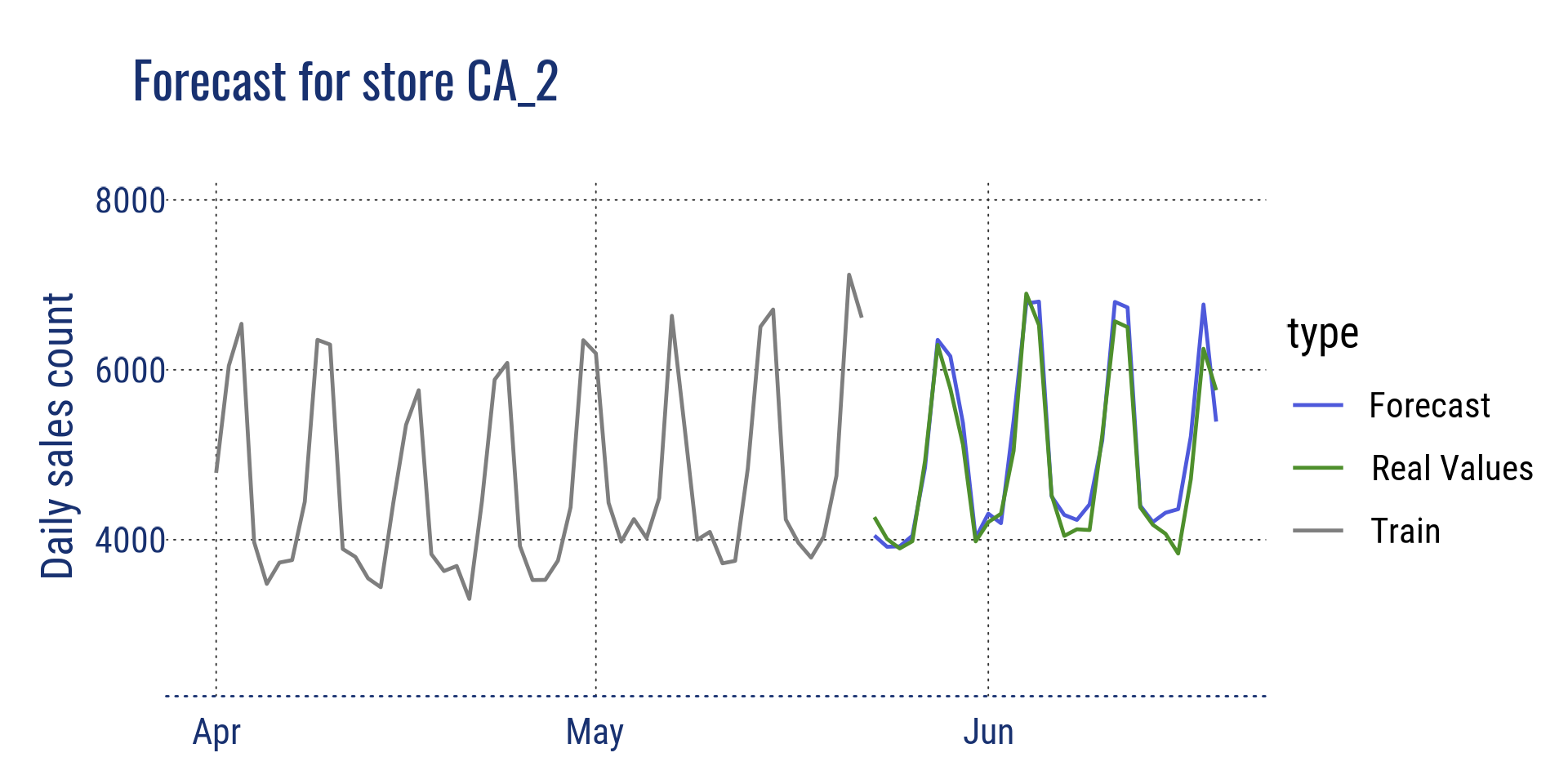
Forecast for store CA_2
Aggregation at category level for store CA_2, and at department level for store CA_2
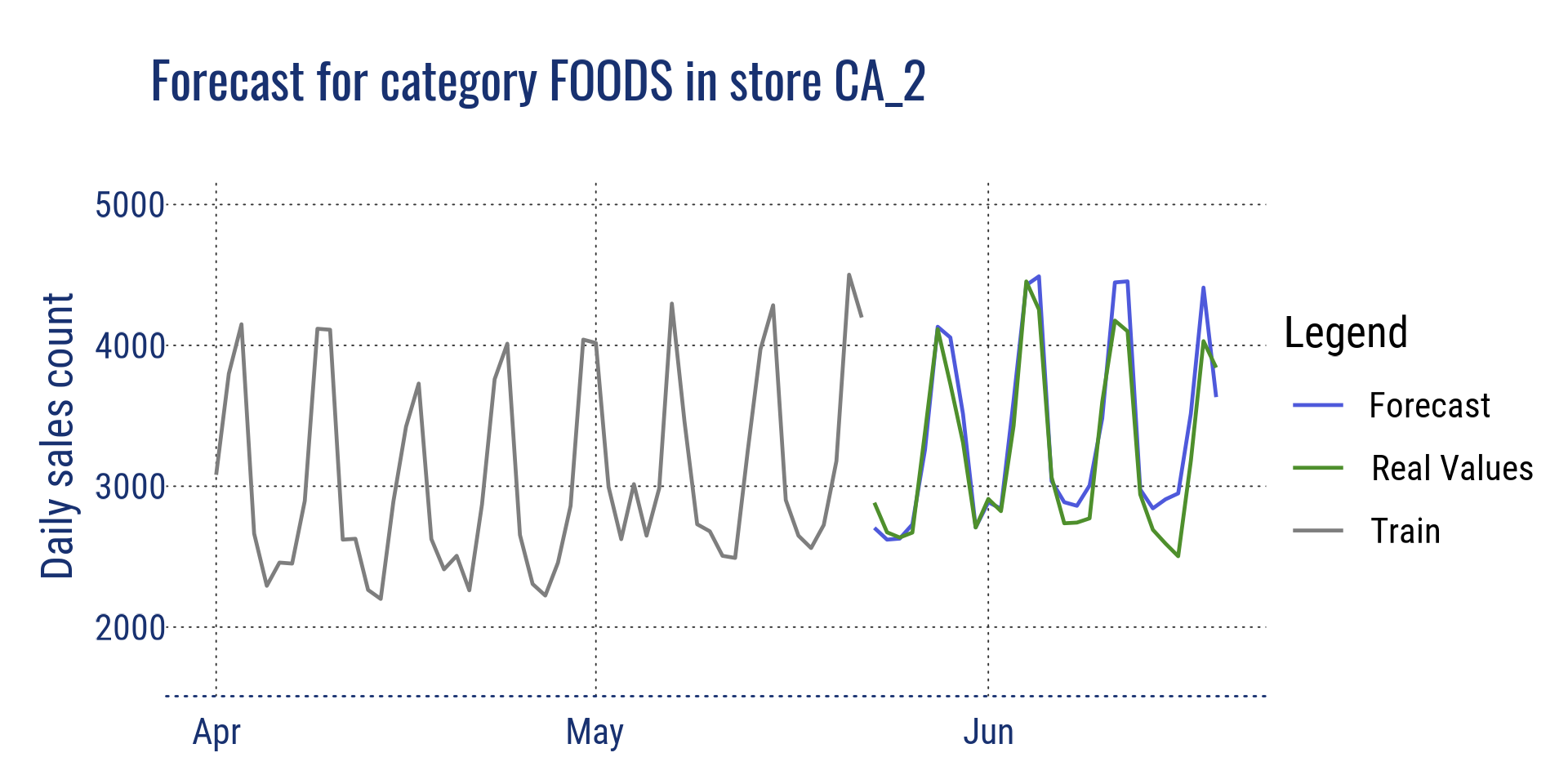
Forecast for category FOODS in the store CA_2
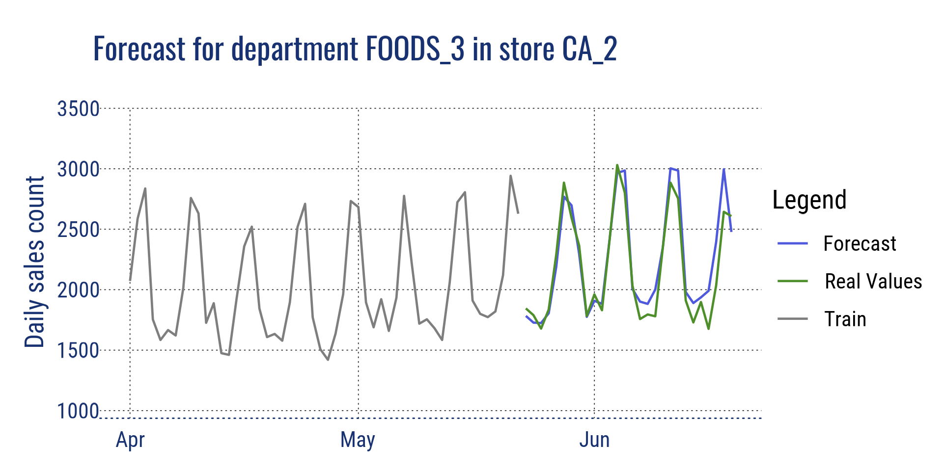
Forecast for department FOODS_3 in CA_2
Aggregation at item level for all stores in California, and for a single item in store CA_2
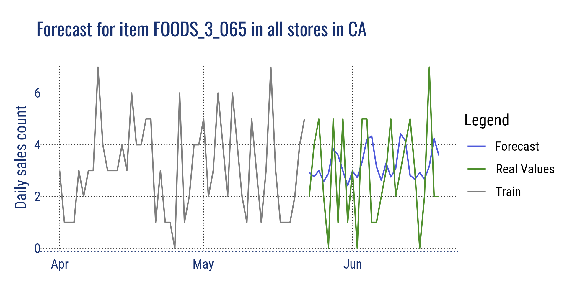
Forecast for item FOODS_3_065 in all stores in CA
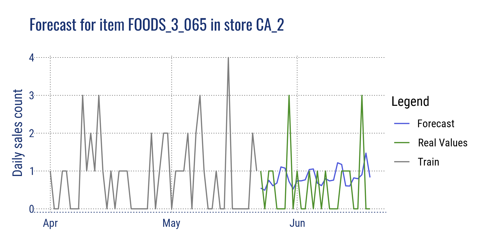
Forecast for item FOODS_3_065 in CA_2
References
My solution for the competition: https://github.com/cnicault/m5-forecasting-accuracy
Competition on Kaggle: https://www.kaggle.com/c/m5-forecasting-accuracy/overview
Winning methods (Python): https://github.com/Mcompetitions/M5-methods
Dataset with the real values: https://drive.google.com/drive/folders/1D6EWdVSaOtrP1LEFh1REjI3vej6iUS_4?usp=sharing
LightGBM: https://lightgbm.readthedocs.io/en/latest/
Christophe Nicault
Information System Strategy
Digital Transformation
Data Science
I work on information system strategy, IT projects, and data science.