Predict missing values
Missing values
As soon as we have to collect and analyze data, we are quickly confronted with the problem of missing data.
What to do ?
There are different possibilities to deal with this missing data, depending on the problem, data type, volume, etc.
For instance :
- Drop observations with missing data (be careful if they are not missing at random).
- Impute the missing values with the average value, median etc.
- For time series data, impute with the last value, or the next value.
- The missing value can be information in itself, it is then interesting to keep the information to analyze the data by creating a new variable for example missing yes/no, that can be used in the analysis.
- Create an algorithm to predict the missing value using the values of other variables.
In this post, I will describe the last method, show how to use deep learning to predict the missing values of a dataset, containing a million observations with a million missing values spread over a set of variables.
For this, I will use data from Kaggle for the June 2022 competition.
Note: I will independently use “missing value” or NA (not available)
You can find the data at the following address: https://www.kaggle.com/competitions/tabular-playground-series-jun-2022/data
Data mining
The dataset consists of 80 variables (plus an id), divided into 4 groups F_1*, F_2*, F_3* et F_4*.
skimr::skim(data) skim_variable n_missing complete_rate mean sd p0 p25 p50 p75 p100 hist
1 row_id 0 1 5.00e+5 288675. 0 250000. 5.00e+5 749999. 999999 ▇▇▇▇▇
2 F_1_0 18397 0.982 -6.87e-4 1.00 -4.66 -0.675 -7.69e-4 0.673 5.04 ▁▂▇▂▁
3 F_1_1 18216 0.982 2.09e-3 1.00 -4.79 -0.672 2.05e-3 0.676 5.04 ▁▂▇▂▁
4 F_1_2 18008 0.982 5.51e-4 1.00 -4.87 -0.674 1.39e-3 0.674 5.13 ▁▂▇▂▁
5 F_1_3 18250 0.982 9.82e-4 1.00 -5.05 -0.672 3.7 e-4 0.675 5.46 ▁▂▇▁▁
6 F_1_4 18322 0.982 2.44e-3 1.00 -5.36 -0.672 2.73e-3 0.677 4.86 ▁▁▇▂▁
7 F_1_5 18089 0.982 6.35e-4 1.00 -5.51 -0.674 2.76e-4 0.676 4.96 ▁▁▇▂▁
8 F_1_6 18133 0.982 -1.24e-4 1.00 -5.20 -0.675 8.14e-4 0.674 4.96 ▁▂▇▂▁
9 F_1_7 18128 0.982 -6.39e-2 0.726 -6.99 -0.500 5.78e-4 0.444 2.53 ▁▁▁▇▂
10 F_1_8 18162 0.982 -1.38e-5 1.00 -4.57 -0.674 -4.7 e-5 0.674 4.89 ▁▂▇▂▁
11 F_1_9 18249 0.982 4.51e-4 1.00 -5.00 -0.674 1.12e-3 0.676 4.79 ▁▂▇▂▁
12 F_1_10 17961 0.982 1.85e-4 0.999 -4.79 -0.674 6.71e-4 0.674 4.91 ▁▂▇▂▁
13 F_1_11 18170 0.982 -1.13e-3 1.00 -4.61 -0.677 -1.29e-3 0.674 4.82 ▁▂▇▂▁
14 F_1_12 18203 0.982 -6.12e-2 0.712 -7.06 -0.489 5.47e-4 0.436 2.30 ▁▁▁▇▃
15 F_1_13 18398 0.982 -6.71e-2 0.746 -6.90 -0.514 -8.04e-4 0.455 2.54 ▁▁▁▇▂
16 F_1_14 18039 0.982 -9.05e-4 1.00 -4.63 -0.676 -1.61e-4 0.673 4.82 ▁▂▇▂▁
17 F_2_0 0 1 2.69e+0 1.88 0 1 2 e+0 4 15 ▇▃▁▁▁
18 F_2_1 0 1 2.51e+0 1.75 0 1 2 e+0 4 14 ▇▆▁▁▁
19 F_2_2 0 1 9.77e-1 1.04 0 0 1 e+0 2 11 ▇▁▁▁▁
20 F_2_3 0 1 2.52e+0 1.65 0 1 2 e+0 4 14 ▇▆▁▁▁
21 F_2_4 0 1 2.94e+0 1.98 0 1 3 e+0 4 16 ▇▃▁▁▁
22 F_2_5 0 1 1.53e+0 1.35 0 1 1 e+0 2 12 ▇▂▁▁▁
23 F_2_6 0 1 1.49e+0 1.32 0 0 1 e+0 2 12 ▇▂▁▁▁
24 F_2_7 0 1 2.65e+0 1.74 0 1 2 e+0 4 16 ▇▃▁▁▁
25 F_2_8 0 1 1.18e+0 1.32 0 0 1 e+0 2 13 ▇▁▁▁▁
26 F_2_9 0 1 1.11e+0 1.10 0 0 1 e+0 2 11 ▇▁▁▁▁
27 F_2_10 0 1 3.28e+0 1.87 0 2 3 e+0 4 17 ▇▅▁▁▁
28 F_2_11 0 1 2.47e+0 1.60 0 1 2 e+0 3 13 ▇▆▁▁▁
29 F_2_12 0 1 2.76e+0 1.70 0 2 3 e+0 4 15 ▇▃▁▁▁
30 F_2_13 0 1 2.48e+0 1.65 0 1 2 e+0 3 15 ▇▂▁▁▁
31 F_2_14 0 1 1.72e+0 1.56 0 1 1 e+0 3 13 ▇▂▁▁▁
32 F_2_15 0 1 1.78e+0 1.46 0 1 2 e+0 3 13 ▇▃▁▁▁
33 F_2_16 0 1 1.80e+0 1.46 0 1 2 e+0 3 13 ▇▃▁▁▁
34 F_2_17 0 1 1.24e+0 1.25 0 0 1 e+0 2 12 ▇▁▁▁▁
35 F_2_18 0 1 1.56e+0 1.44 0 0 1 e+0 2 15 ▇▁▁▁▁
36 F_2_19 0 1 1.60e+0 1.42 0 0 1 e+0 2 13 ▇▂▁▁▁
37 F_2_20 0 1 2.23e+0 1.56 0 1 2 e+0 3 14 ▇▅▁▁▁
38 F_2_21 0 1 2.03e+0 1.61 0 1 2 e+0 3 15 ▇▂▁▁▁
39 F_2_22 0 1 1.61e+0 1.56 0 0 1 e+0 2 16 ▇▁▁▁▁
40 F_2_23 0 1 7.09e-1 1.08 0 0 0 1 11 ▇▁▁▁▁
41 F_2_24 0 1 3.13e+0 1.82 0 2 3 e+0 4 17 ▇▅▁▁▁
42 F_3_0 18029 0.982 1.74e-3 1.00 -4.69 -0.675 3.25e-3 0.677 4.59 ▁▂▇▂▁
43 F_3_1 18345 0.982 -1.15e-3 1.00 -4.47 -0.675 4.81e-4 0.674 4.85 ▁▃▇▂▁
44 F_3_2 18056 0.982 6.05e-4 0.999 -4.89 -0.673 3.92e-4 0.675 4.76 ▁▂▇▂▁
45 F_3_3 18054 0.982 8.34e-4 1.00 -4.68 -0.674 8.54e-4 0.676 4.99 ▁▂▇▂▁
46 F_3_4 18373 0.982 1.29e-3 1.00 -5.01 -0.673 2.64e-3 0.677 4.72 ▁▂▇▂▁
47 F_3_5 18298 0.982 -2.18e-3 1.00 -4.87 -0.676 -1.60e-3 0.672 5.04 ▁▂▇▂▁
48 F_3_6 18192 0.982 5.78e-5 0.999 -5.02 -0.675 8.54e-4 0.673 4.53 ▁▂▇▃▁
49 F_3_7 18013 0.982 1.52e-3 1.00 -5.05 -0.673 1.20e-3 0.676 5.46 ▁▂▇▁▁
50 F_3_8 18098 0.982 7.73e-4 1.00 -5.51 -0.676 -1.95e-5 0.676 5.11 ▁▁▇▂▁
51 F_3_9 18106 0.982 -4.40e-4 1.00 -4.85 -0.675 -1.77e-3 0.674 5.10 ▁▂▇▂▁
52 F_3_10 18200 0.982 1.71e-3 1.00 -4.63 -0.672 1.57e-3 0.675 5.13 ▁▃▇▁▁
53 F_3_11 18388 0.982 7.33e-4 0.999 -4.60 -0.675 4.80e-4 0.675 4.68 ▁▂▇▂▁
54 F_3_12 18297 0.982 2.59e-4 1.00 -4.53 -0.674 1.83e-3 0.674 4.94 ▁▃▇▂▁
55 F_3_13 18060 0.982 -2.46e-3 1.00 -4.75 -0.676 -1.59e-3 0.674 4.71 ▁▂▇▂▁
56 F_3_14 18139 0.982 7.27e-4 0.999 -5.36 -0.673 1 e-4 0.674 4.82 ▁▁▇▃▁
57 F_3_15 18238 0.982 -1.51e-3 1.00 -4.45 -0.675 -1.36e-3 0.674 5.25 ▁▃▇▁▁
58 F_3_16 18122 0.982 -6.65e-4 1.00 -4.82 -0.675 -1.70e-3 0.675 4.84 ▁▂▇▂▁
59 F_3_17 18278 0.982 -2.14e-4 1.00 -4.81 -0.675 -4.14e-4 0.674 5.06 ▁▂▇▂▁
60 F_3_18 18089 0.982 6.27e-5 1.00 -5.20 -0.674 1.63e-4 0.675 4.96 ▁▂▇▂▁
61 F_3_19 18200 0.982 -6.49e-2 0.739 -6.07 -0.507 6.76e-4 0.451 2.67 ▁▁▂▇▁
62 F_3_20 18248 0.982 2.37e-3 0.999 -5.00 -0.671 2.45e-3 0.676 6.03 ▁▃▇▁▁
63 F_3_21 18396 0.982 -5.93e-2 0.697 -7.15 -0.480 -6.49e-4 0.428 2.39 ▁▁▁▇▂
64 F_3_22 18177 0.982 8.73e-5 0.999 -4.74 -0.674 5.9 e-5 0.674 4.97 ▁▂▇▂▁
65 F_3_23 18206 0.982 3.65e-4 1.00 -5.25 -0.674 -4.52e-4 0.675 4.81 ▁▁▇▂▁
66 F_3_24 18145 0.982 -8.17e-4 1.00 -4.89 -0.675 -4.57e-4 0.674 4.98 ▁▂▇▂▁
67 F_4_0 18128 0.982 3.27e-1 2.32 -12.9 -1.17 4.21e-1 1.91 10.7 ▁▁▇▅▁
68 F_4_1 18164 0.982 -3.31e-1 2.41 -12.5 -1.96 -3.56e-1 1.28 11.7 ▁▂▇▂▁
69 F_4_2 18495 0.982 -8.58e-2 0.837 -9.66 -0.608 -6.20e-2 0.485 2.91 ▁▁▁▇▃
70 F_4_3 18029 0.982 -1.95e-1 0.821 -9.94 -0.686 -1.37e-1 0.369 2.58 ▁▁▁▇▅
71 F_4_4 17957 0.982 3.33e-1 2.37 -12.8 -1.19 4.25e-1 1.94 11.9 ▁▁▇▃▁
72 F_4_5 18063 0.982 3.36e-1 2.35 -12.5 -1.27 3.03e-1 1.92 13.5 ▁▂▇▁▁
73 F_4_6 18325 0.982 3.77e-3 2.29 -11.1 -1.57 -7.18e-2 1.52 11.5 ▁▂▇▂▁
74 F_4_7 18014 0.982 3.34e-1 2.36 -11.7 -1.22 3.79e-1 1.93 12.5 ▁▂▇▂▁
75 F_4_8 18176 0.982 -7.18e-2 0.778 -10.1 -0.518 1.82e-2 0.475 2.61 ▁▁▁▇▇
76 F_4_9 18265 0.982 -7.99e-2 0.807 -9.86 -0.577 -2.78e-2 0.480 2.81 ▁▁▁▇▅
77 F_4_10 18225 0.982 3.83e-2 0.707 -10.4 -0.386 1.03e-1 0.530 2.55 ▁▁▁▆▇
78 F_4_11 18119 0.982 5.52e-1 5.00 -26.3 -2.79 2.03e-1 3.65 31.2 ▁▂▇▁▁
79 F_4_12 18306 0.982 3.34e-1 2.38 -11.5 -1.27 3.54e-1 1.95 11.3 ▁▂▇▂▁
80 F_4_13 17995 0.982 3.30e-1 2.36 -10.7 -1.30 2.95e-1 1.92 11.9 ▁▂▇▂▁
81 F_4_14 18267 0.982 3.72e-2 0.776 -9.98 -0.396 1.31e-1 0.574 2.58 ▁▁▁▇▇All variables are continuous except for F_2* variables which do not contain missing data. We must therefore predict the missing for continuous data, it is a regression problem.
Each variable contains approximately the same proportion of missing 1.8%.
How are they distributed?
data$count_na <- rowSums(is.na(data))

data %>%
  count(count_na, sort = TRUE)
count_na n
<dbl> <int>
1 1 370798
2 0 364774
3 2 185543
4 3 61191
5 4 14488
6 5 2723
7 6 413
8 7 64
9 8 4
10 9 2There are 364,774 observations without NA, 370,798 with a single NA, and up to 9 NAs for the same observation.
A strategy can begin to take shape here, which would consist of using the 364,774 observations without missing value to train the algorithm and predict the 370798 with missing. The problem will be more complex from 2 NAs because they will probably not be distributed on the same variables.
If we look at the missing combinations, there are 42633 possible combinations (code to find out all the combination in the section about building the model). We will therefore have to simplify the problem.
Let’s visualize the correlations:
corrplot::corrplot(cor(drop_na(data[,-1])), tl.cex = 0.5, tl.col = "black", method = "color")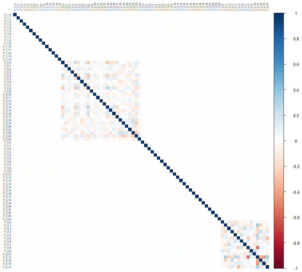
Looking at the correlation matrix, we see that there is no correlation between the groups of variables, and only the groups F_2 and F_4 present correlations but only internal to the group.
This suggests that it will be difficult to predict the F_1* and F_3* variables, and that the F_2* variables will probably not be of much help.
One way to confirm this is to create a first algorithm to predict these variables when there is only one NA. So I quickly created an algorithm that loops on each variable, and created a model (using LightGBM) for each variable to predict. We immediately notice that it does not succeed, and this for each of the variables F_1* and F_3*.
We can immediately see that the RMSE increases for the validation data instead of decreasing:
[1]:  train's rmse:0.99907  valid's rmse:0.999992
[11]:  train's rmse:0.983548  valid's rmse:1.00045
[21]:  train's rmse:0.968703  valid's rmse:1.00171
[31]:  train's rmse:0.954811  valid's rmse:1.00238
[41]:  train's rmse:0.941672  valid's rmse:1.00242
[51]:  train's rmse:0.929105  valid's rmse:1.00233
And by ploting the evolution of the RMSE for train and valid:

We can clearly see on the validation data that the predictions are deteriorating.
The best strategy for the variables F_1* and F_3* is to impute with their means, after some tests, this is what gives the best result. 40 variables can therefore be processed in a very simple way.
See code for imputation with mean or median on github.
All that remains is to find a solution for the F_4* variables, of which there are only 15.
Let’s look again at the correlation matrix just for these variables:
corrplot::corrplot(cor(drop_na(select(data, contains("F_4")))), tl.cex = 0.5, tl.col = "black", method = "square", type = "upper")
corrplot::corrplot.mixed(cor(drop_na(select(data, contains("F_4")))), tl.cex = 0.5, tl.col = "black", tl.offset = 0.2, upper = "color", number.cex = 0.8, tl.pos = "lt")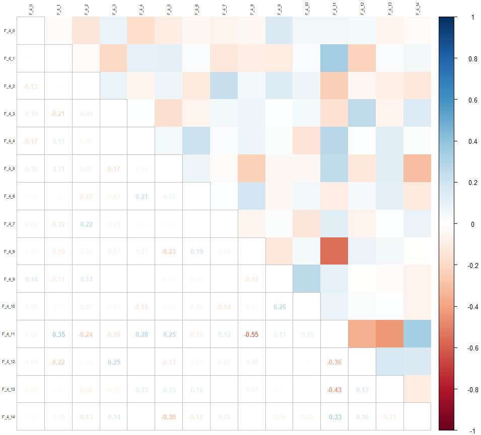
We re-evaluate the missing values only for these variables:
   count_na      n
      <dbl>  <int>
1         0 759268
2         1 211342
3         2  27127
4         3   2124
5         4    135
6         5      4
We only have a maximum of 5 missing per observation, and a proportion of complete data to train the algorithm of 76%.
Of course, when there is more than one missing, they can be distributed over 14 variables, which in our case gives 703 combinations.
For example, to predict the missing of the variable F_4_0, we can have no other missing, or one missing on the variable F_4_2, or on the variable F_4_3, or even 2 other missing, on the variables F_4_3 and F_4_5 etc.
Strategies
Strategy 1: Prediction by variable
The principle is to use an algorithm that can make predictions despite missing values, such as LightGBM. We create a model for each variable to be predicted, which we train on the data that has no gaps.
All missing values of this variable are predicted regardless of whether values of other variables may be missing. Of course, the more missing values there are, the worse the prediction will be. We can play on certain lightGBM parameters to improve tolerance to missing items such as feature_fraction which reduces the number of variables used for each decision tree. This can be tricky, as it can reduce performance for full observations. It is therefore necessary to find the right value of the parameter by hyperparameter tuning.
To improve the predictions, we can complete with a neural network: we then use a second dataframe whose missing values have been replaced by those predicted by lightGBM (neural networks cannot manage NA).
- Pros: we only created 15 models, so it’s quite fast, the RMSE is 0.86 which is correct
- Cons: lightGBM predictions are more imprecise when there are missing values, and these values are used by the neural network, so we can amplify the uncertainty and the margin for improvement is small.
Strategy 2: Alter training data to add a value for NA replacement
This strategy was proposed by one of the competitors on Kaggle. This involves replacing the NAs with a value (-1 but you can choose something else) for the independent variables in order to be able to use deep learning. But of course we cannot make a prediction if these values have not been seen beforehand during the training phase. It is therefore necessary to alter the training data to replace real data randomly with -1.
For it to work, you have to add as many -1 as there are NAs, so we create models by number of NAs in the independent variables. For example if there are 2 independent variables with NA, we create for each observation of the training data, 2 values -1 which we distribute randomly between the variables by ensuring that there are only 2 NA per observation.
- Pros: it slightly improves the predictions
- Cons: It is more complex to code (in particular to randomly assign the -1 according to the number of NA), and longer to train.
Strategy 3: Predict multiple variables simultaneously (regression with multiple outputs)
This is the strategy that gave the best result and that I will then explain in this post.
The idea here is to predict for each combination of NAs, a model that will have as many outputs as missing values to predict all the missing values simultaneously.
It’s finally quite easy to do, because it involves creating a neural network with as many neurons as there are NAs for the output layer.
Implementation
To be able to apply this strategy, the data must be grouped by combination of missing values. We therefore create a variable which lists the names of the variables containing NA for each observation.
list_variables <- colnames(data)
list_cols <- list_variables[grep("F_4",list_variables)]

data <- data %>%
   select(row_id, all_of(list_cols))
We create a na_col() function which creates a new variable containing the name of the variable if the value of the original variable is NA, or empty otherwise.
na_col <- function(var, data){

  var_ts <- sym(var)
  new_var_ts <- sym(glue::glue(var, "_na"))

  data %>%
    select({{var_ts}}) %>%
    mutate("{{new_var_ts}}" := ifelse(is.na({{var_ts}}), var, "")) %>%
    select(-{{var_ts}})

}
We use map_dfr() and reduce() from the {purrr} package to apply the na_col() function to all the variables and obtain a single variable with the list of all the variables containing NAs per observation.
data_mut <- map_dfc(list_cols, na_col, data) %>%
  mutate(na_cols = reduce(., paste, sep = " ")) %>%
  mutate(na_cols = str_squish(na_cols))

data <- data %>%
  bind_cols(select(data_mut, na_cols))

data$cnt <- rowSums(is.na(data))   # nb NA
Explanation :
map_dfc()applies thena_col()function on all variables and returns a dataframe containing as many columns as there are variables, and containing the name of the variable if its value is NA, or empty otherwise .reduce()combined withpaste, allows to create only one variable containing the concatenation of all these values.str_squish()removes all extra spaces, keeping only the separators.
We now have a dataframe containing only the F_4_* variables as well as the na_cols variable, which contains the list of variables containing NAs, separated by a space, and the cnt variable which contains the number of NAs per observation .
Let’s look at an overview of the number of unique combinations:
unique_combi <- unique(data$na_cols)[-1]
head(unique_combi, 20)
[1] "F_4_2" "F_4_4" "F_4_3 F_4_14" "F_4_12" "F_4_14" "F_4_3" "F_4_8 F_4_12" "F_4_1" "F_4_8 F_4_14"
[10] "F_4_8" "F_4_4 F_4_14" "F_4_5" "F_4_9" "F_4_2 F_4_13" "F_4_10" "F_4_3 F_4_13" "F_4_0" "F_4_7 F_4_9"
[19] "F_4_6" "F_4_13"
We then use the part of the dataframe containing no NA to train the algorithm, with a split to have training and validation data.
train_basis <- data %>%
  filter(cnt == 0) %>%
  select(-na_cols, -cnt)

split <- floor(0.80*NROW(train_basis))
We can then loop over all the combinations of variables to create as many models as there are combinations. However, given the number of models to be created, it is preferable to loop by variable to be predicted, and then by combination comprising this variable, which makes it possible to run several models in parallel. This is what this structure does:
for(variable in list_cols){

  combi_var <- unique_combi[str_detect(unique_combi, variable)]

  for(combi in combi_var){

    set_cols <- str_split(combi, " ", simplify = TRUE)[,1]

    # ** MODEL **

  }

}
The set_cols variable contains the list of columns containing NAs for this iteration of the loop.
So we can focus on the model.
The training data contains all the columns not containing missing, and the target is a matrix containing the values for the different variables to be predicted (those contained in set_cols)
train_df <- train_basis[1:split,] %>%
   select(-all_of(set_cols), -row_id)
train_target <- train_basis[1:split,] %>%
   select(all_of(set_cols)) %>%
   as.matrix()
We do the same for the validation data:
valid_df <- train_basis[split:NROW(train_basis),] %>%
  select(-all_of(set_cols), -row_id)
valid_target <- train_basis[split:NROW(train_basis),] %>%
  select(all_of(set_cols)) %>%
  as.matrix()
And finally we prepare the test data by filtering only the data containing NA for this combination of variable, and by selecting only the variables which have no missing value:
test_df <- data %>%
  filter(na_cols %in% combi) %>%
  select(-all_of(set_cols), -cnt, -na_cols)

test_row_id <- test_df$row_id
test_df <- test_df %>% select(-row_id)
We normalize the data:
preProcValues <- caret::preProcess(select(train_basis[-1], -all_of(set_cols)), method = c("center", "scale"))

trainTransformed <- predict(preProcValues, train_df)
validTransformed <- predict(preProcValues, valid_df)
testTransformed <- predict(preProcValues, test_df)

train_mx <- as.matrix(trainTransformed)
We define the model with an input layer comprising as many neurons as there are variables without NA, and in the output layer as many neurons as there are variables with NAs. This model will therefore produce a matrix comprising one column per variable to be predicted.
model <- keras_model_sequential() %>%
  layer_dense(units = 128, activation = "swish", input_shape = length(train_df)) %>%
  layer_batch_normalization() %>%
  layer_dense(units = 64, activation = "swish") %>%
  layer_dense(units = 32, activation = "swish") %>%
  layer_dense(units = 8, activation = "swish") %>%
  layer_dense(length(set_cols), activation = "linear")
We define the optimizer and we can compile the model with the loss function and metric “mean_squared_error”.
optimizer <- optimizer_adam(learning_rate = 0.001)

model %>%
  compile(
    loss = 'mean_squared_error',
    optimizer = optimizer,
    metrics = "mean_squared_error"
  )
Finally, we can train the model using the fit() function, passing the data, the number of epochs and the batch size as parameters. We also define two callback functions, one to stop training if there is no improvement (early stopping) and one to reduce the learning rate if a plateau is reached (reduce lr on plateau) .
model %>% fit(
  train_mx,
  train_target,
  epochs = EPOCHS,
  batch_size = BATCH_SIZE,
  validation_split = 0.1,
  callbacks = list(
    callback_early_stopping(monitor='val_mean_squared_error', patience=8, verbose = 1, mode = 'min', restore_best_weights = TRUE),
    callback_reduce_lr_on_plateau(monitor = "val_loss", factor = 0.5, patience = 3, verbose = 1)
  )
)
We then make predictions on the validation data to evaluate the RMSE on these data that the algorithm has not seen.
pred_valid <- model %>% predict(as.matrix(validTransformed))

predictions_valid <- as.data.frame(pred_valid)
colnames(predictions_valid) <- set_cols
predictions_valid <- predictions_valid %>%
  mutate(row_id = row_number()) %>%
  pivot_longer(cols = -row_id)
valid_target <- as.data.frame(valid_target) %>%
  mutate(row_id = row_number()) %>%
  pivot_longer(cols = -row_id)

rmse <- yardstick::rmse_vec(valid_target$value, predictions_valid$value)
print(glue("RMSE - combination {reduce(combi, paste, sep = ", ")}: {rmse}"))
Which produces:
...
RMSE - combination F_4_8 F_4_10 F_4_14: 0.296459822230795
RMSE - combination F_4_6 F_4_7 F_4_10: 0.798801761253467
RMSE - combination F_4_0 F_4_2 F_4_13: 0.68729877310422
RMSE - combination F_4_2 F_4_7 F_4_8 F_4_10: 0.727564592227748
RMSE - combination F_4_4 F_4_6 F_4_10 F_4_11: 1.13184400510586
RMSE - combination F_4_1 F_4_9 F_4_10 F_4_11: 0.815886927914656
...
Finally, we predict on the test data which are the true missing data to be predicted, then we format the predictions to add to the file each variable / id pair with the predicted value.
    test_predictions <- model %>% predict(as.matrix(testTransformed))
    test_predictions <- as.data.frame(test_predictions)
    colnames(test_predictions) <- set_cols
    test_predictions$row_id <- test_row_id

    test_predictions <- test_predictions %>%
      pivot_longer(cols = -row_id, names_to = "variable", values_to = "prediction")


    predictions <- tibble(`row-col` = glue("{test_predictions$row_id}-{test_predictions$variable}"), value = test_predictions$prediction)

    submission <- submission %>% bind_rows(predictions)
Conclusion
Voilà! We have just predicted a million missing values in a table containing a million rows and 80 variables.
There is a noticeable difference between the first solution using LightGBM and the use of a multi-output neural network, but the first solution requires about 2 hours of training, while the last one requires almost 30 hours (without GPU). The difference is significant in the context of a competition, in practice perhaps less, it is to be defined according to the problem, and the first solution gives a satisfactory result compared to an imputation with the average.
As a benchmark, here is the RMSE for different strategies:
- Imputation with the mean: 0.97937
- LGBM + NN: 0.85xx
- Alteration: 0.84xx
- Multi-output NN: 0.83xx
Knowing how to impute missing values is useful to be able to carry out an analysis despite the absence of certain data, which is a very frequent problem in practice.
Références
My solution for the competition: https://github.com/cnicault/tabular-playground-series/tree/main/Jun-2022
Competition on Kaggle: https://www.kaggle.com/competitions/tabular-playground-series-jun-2022/data
Christophe Nicault
Information System Strategy
Digital Transformation
Data Science
I work on information system strategy, IT projects, and data science.